Example Using a Holdback Set
In this Time Series example, use a holdback set to evaluate predictions made on monthly data on lead production. Since a holdback set is used, both State Space Smoothing and ARIMA models can be fit and compared to find the best fitting model for the data.
1. Select Help > Sample Data Folder and open Time Series/Lead Production.jmp.
2. Select Analyze > Specialized Modeling > Time Series.
3. Select LEADPROD and click Y, Time Series.
4. Select DATE and click X, Time ID.
5. Select Forecast on Holdback.
Selecting this option means that forecasts are made on the holdback set instead of on future observations.
6. Enter 12 next to Forecast Periods.
This assigns the last 12 observations in the data to the holdback set. Since this is monthly data, this is equivalent to the last year.
7. Click OK.
8. Click the Time Series LEADPROD red triangle and select State Space Smoothing.
9. Type 12 next to Period.
10. Select Constrain Parameters.
11. Click OK.
12. Click the Time Series LEADPROD red triangle and select ARIMA Model Group.
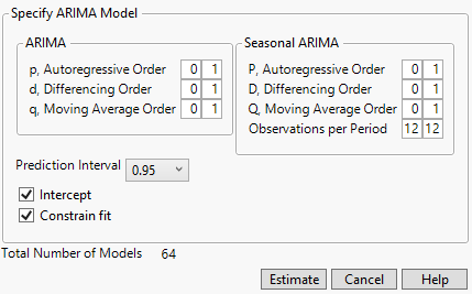
13. Set the range for all parameters from 0 to 1. The Specify ARIMA Model window looks like the one in Figure 18.24.
Figure 18.24 ARIMA Model Group Specifications
14. Click Estimate.
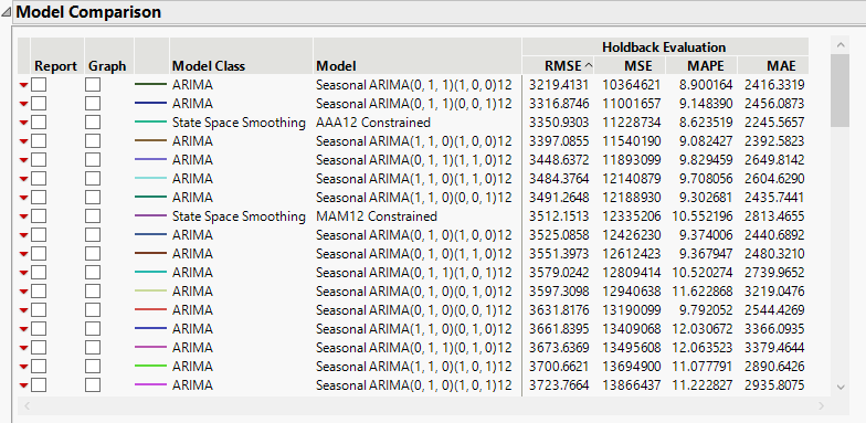
Figure 18.25 Model Comparison
The fit statistics are comparable between the State Space Smoothing models and the ARIMA models because they are evaluated on the holdback set.
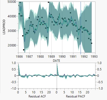
15. Select the Graph check box next to the first three models in the Model Comparison report.
Figure 18.26 Model Comparison Graph
The evaluation statistics and the forecasting plots show that there is no substantial differences in forecasting performance among the top models. Based on the report, either an ARIMA model or a State Space Smoothing model is appropriate for this data.


