Example Using Standard Least Squares
This example shows how to use the Standard Least Squares personality of the Fit Model platform to fit an analysis of covariance model. In a study of the effect of drugs in treating a disease, thirty patients are randomly divided into three groups of ten. Two of these groups are administered drugs (Drug a and Drug d), whereas the third group is administered a placebo (Drug f). A pretreatment measure, x, is taken on each patient, as well as a posttreatment measure, y. The pretreatment score, x, is included as a covariate, to account for differences in the stage of the disease among patients.
You are interested in determining if there is a difference in the three Drug groups. You construct a model with response y and model effects Drug, x, and the interaction of Drug and x. The interaction might account for a situation where drugs have differential effects, based on the stage of the disease. For background on the Fit Model window and the various personalities, see Model Specification.
1. Select Help > Sample Data Folder and open Drug.jmp.
2. Select Analyze > Fit Model.
3. Select y and click Y.
When you add this column as Y, the fitting Personality becomes Standard Least Squares. An Emphasis option is added with a selection of Effect Leverage, which you can change if desired.
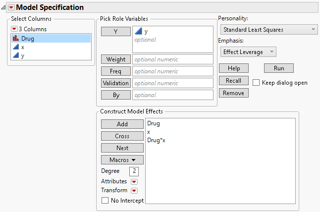
4. Select Drug and x. With these two effects highlighted in the Select Columns list, click Macros and select Full Factorial. The macro adds the two effects and their two-way interaction to the Construct Model Effects list.
Figure 3.2 Completed Fit Model Launch Window
5. Click Run.
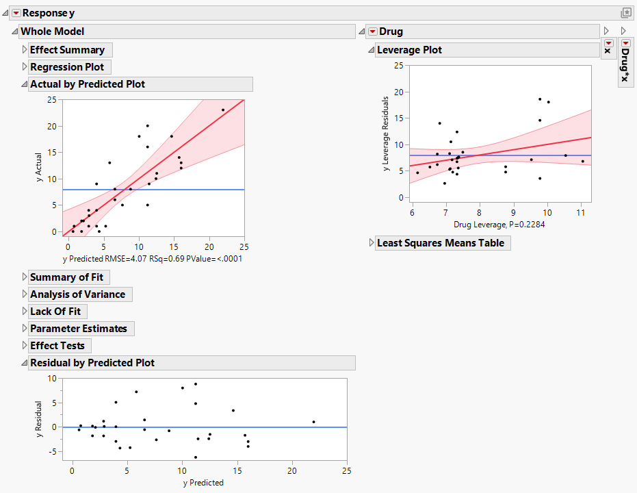
The Fit Least Squares report is shown in Figure 3.3. Note that some of the constituent reports are closed because of space considerations. The Actual by Predicted, Residual by Predicted, and Leverage plots show no discrepancies in terms of model fit and underlying assumptions.
Figure 3.3 Fit Least Squares Report Showing Plots to Assess Model Fit
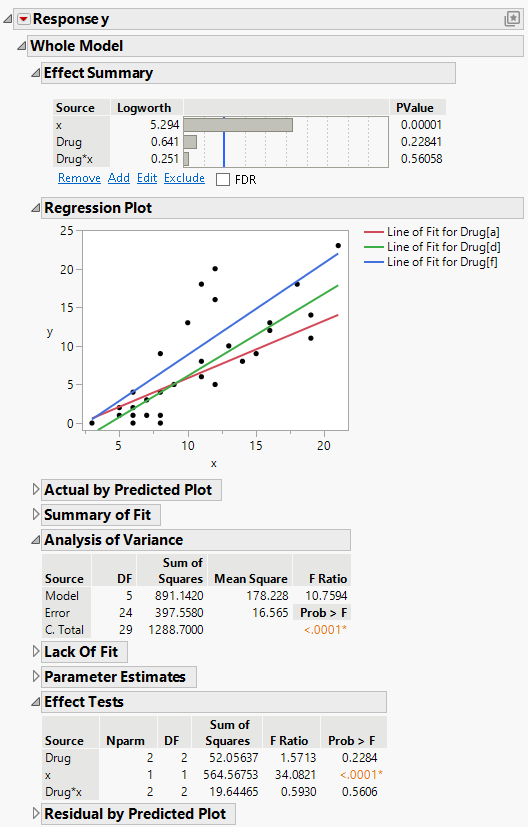
Since there are no apparent problems with the model fit, you can now interpret the statistical tests. Figure 3.4 shows the relevant reports. The overall model is significant, as shown in the Analysis of Variance report.
Although the Regression Plot suggests that Drug and the pretreatment measure, x, interact, the Prob > F value in the Effect Tests report does not support that conclusion. The Effect Tests report also shows that x is significant in explaining y, but Drug is not significant. The study does not detect a difference among the three groups. However, you cannot conclude that Drug has no effect. The drugs might have different effects, but the study size was not large enough to detect that difference.
Figure 3.4 Fit Least Squares Report Showing Reports to Assess Significance


