Statistical Details for Discrete Fit Distributions
This section contains statistical details for the options in the Discrete Fit menu in the Distribution platform. Unless otherwise specified, confidence intervals for parameter estimates use likelihood-based calculations. For more information about likelihood-based confidence intervals, see Statistical Details for Profile Likelihood Confidence Limits in Predictive and Specialized Modeling.
Fit Poisson
The Poisson distribution has a single scale parameter λ > 0.
pmf:  for 0 ≤ λ < ∞; x = 0,1,2,...
E(x) = λ
Var(x) = λ
Since the Poisson distribution is a discrete distribution, the overlaid curve is a step function, with jumps that occur at every integer.
Fit Negative Binomial
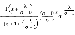
The negative binomial distribution is useful for modeling the number of successes before a specified number of failures. The following parameterization contains mean parameter λ and dispersion parameter σ.
pmf: 
E(x) = λ
Var(x) = λ + σλ2
where Γ(·) is the Gamma function.
Relationship between Negative Binomial and Gamma Poisson Distributions
The negative binomial distribution is equivalent to the Gamma Poisson distribution. The Gamma Poisson distribution is useful when the data are a combination of several Poisson(μ) distributions and each Poisson(μ) distribution has a different μ.
The Gamma Poisson distribution results from assuming that x|μ follows a Poisson distribution and μ follows a Gamma(α,τ). The Gamma Poisson has parameters λ = ατ and σ = τ+1. The parameter σ is a dispersion parameter. If σ > 1, there is over dispersion, meaning there is more variation in x than explained by the Poisson alone. If σ = 1, x reduces to Poisson(λ).
pmf:  for 0 < λ; 1 ≤ σ; x = 0,1,2,...
E(x) = λ
Var(x) = λσ
where Γ(·) is the Gamma function.
The Gamma Poisson is equivalent to a Negative Binomial with σnegbin = (σgp - 1) / λgp.
Run demoGammaPoisson.jsl in the JMP Samples/Scripts folder to compare a Gamma Poisson distribution with parameters λ and σ to a Poisson distribution with parameter λ.
Fit ZI Poisson
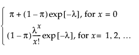
The zero-inflated (ZI) Poisson distribution has scale parameter λ > 0 and zero-inflation parameter π.
pmf: 
E(x) = (1 - π)λ
Var(x) = λ(1 - π)(1 + λπ)
Fit ZI Negative Binomial
The zero-inflated (ZI) negative binomial distribution has scale parameter λ > 0, dispersion parameter σ > 0, and zero-inflation parameter π.
pmf: 
E(x) = (1 - π)λ
Var(x) = λ(1 - π)[1 + λ(σ + π)]
Fit Binomial
The Fit Binomial option accepts data in two formats: a constant sample size, or a column containing sample sizes.
pmf:  for 0 ≤ p ≤ 1; x = 0,1,2,...,n
E(x) = np
Var(x) = np(1-p)
where n is the number of independent trials.
Note: The confidence interval for the binomial parameter is a profile likelihood interval.
Fit Beta Binomial
The beta binomial distribution is useful when the data are a combination of several Binomial(p) distributions and each Binomial(p) distribution has a different p. One example is the overall number of defects combined from multiple manufacturing lines, when the mean number of defects (p) varies between the lines.
The beta binomial distribution results from assuming that x|π follows a Binomial(n,π) distribution and π follows a Beta(α,β). The beta binomial has parameters p = α/(α+β) and δ = 1/(α+β+1). The parameter δ is a dispersion parameter. When δ > 0, there is over dispersion, meaning there is more variation in x than explained by the Binomial alone. When δ < 0, there is under dispersion. When δ = 0, x is distributed as Binomial(n,p). The beta binomial exists only when n ≥ 2.
pmf: 
for  ;
;  ; x = 0,1,2,...,n
E(x) = np
Var(x) = np(1-p)[1+(n-1)δ]
where Γ(·) is the Gamma function.
Remember that x|π ~ Binomial(n,π), while π ~ Beta(α,β). The parameters p = α/(α+β) and δ = 1/(α+β+1) are estimated by the platform. To obtain estimates of α and β, use the following formulas:


If the estimate of δ is 0, the formulas do not work. In that case, the beta binomial has reduced to the Binomial(n,p), and  is the estimate of p.
The confidence intervals for the beta binomial parameters are profile likelihood intervals.
Run demoBetaBinomial.jsl in the JMP Samples/Scripts folder to compare a beta binomial distribution with dispersion parameter δ to a Binomial distribution with parameters p and n = 20.
Fit ZI Binomial
The Fit ZI Binomial option accepts data in two formats: a constant sample size, or a column containing sample sizes.
pmf: 
E(x) = (1-π)np
Var(x) = (1-π)[np(1-p) + n2p2] - [(1-π)np]2
where n is the number of independent trials.
Fit ZI Beta Binomial
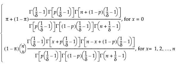
The Fit ZI Beta Binomial option accepts data in two formats: a constant sample size, or a column containing sample sizes. The ZI beta binomial exists only when n ≥ 2.
pmf: 
E(x) = (1-π)np
Var(x) = (1-π)np[(1-p)(1 + (n-1)δ) + np] - [(1-π)np]2
where n is the number of independent trials.