Statistical Details for Fit Curve Models

Predictive and Specialized Modeling > Fit Curve > Statistical Details for the Fit Curve Platform > Statistical Details for Fit Curve Models

Publication date: 07/08/2024

Statistical Details for Fit Curve Models

The formulas for the models that are available in the Fit Curve red triangle menu are summarized in Table 14.1.

Table 14.1 Fit Curve Model Formulas
Model	Formula
Polynomials	where k is the order of the polynomial. These models can also be fit using the Fit Model and Fit Y by X platforms.
Power Model	a = Intercept b = Slope c = Power Available only when both the response values and the x values are nonnegative.
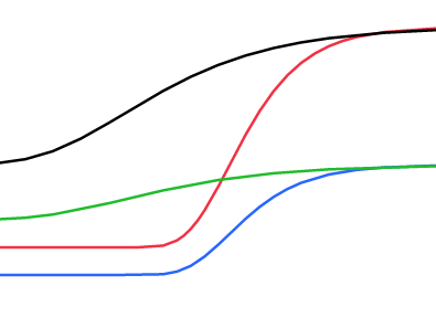
Logistic 2P	a = Growth Rate b = Inflection Point Available only when all response values are between zero and one.
Logistic 3P	a = Growth Rate b = Inflection Point c = Asymptote
Logistic 4P	a = Growth Rate b = Inflection Point c = Lower Asymptote d = Upper Asymptote
Logistic 4P Rodbard	a = Growth Rate b = Location c = Lower Asymptote d = Upper Asymptote Available only when the x values are positive.
Logistic 4P Hill	a = Growth Rate b = Inflection Point c = Lower Asymptote d = Upper Asymptote
Logistic 5P	a = Growth Rate b = Location c = Asymptote 1 d = Asymptote 2 f = Power
Probit 2P	a = Growth Rate b = Inflection Point Φ = Normal Distribution CDF Available only when all response values are between zero and one.
Probit 3P	a = Growth Rate b = Inflection Point c = Asymptote Φ = Normal Distribution CDF There is also an asymptote at zero.
Probit 4P	a = Growth Rate b = Inflection Point c = Lower Asymptote d = Upper Asymptote Φ = Normal Distribution CDF
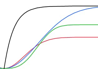
Gompertz 3P	a = Asymptote b = Growth Rate c = Inflection Point
Gompertz 4P	a = Lower Asymptote b = Upper Asymptote c = Growth Rate d = Inflection Point
Weibull Growth	a = Upper Asymptote b = Location c = Growth Rate Available only when both the response values and the x values are nonnegative.
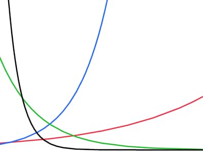
Exponential 2P	a = Scale b = Growth Rate
Exponential 3P	a = Asymptote b = Scale c = Growth Rate
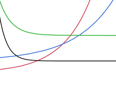
Biexponential 4P	a = Scale 1 b = Decay Rate 1 c = Scale 2 d = Decay Rate 2 Available only when the response values are positive.
Biexponential 5P	a = Asymptote b = Scale 1 c = Decay Rate 1 d = Scale 2 f = Decay Rate 2
Mechanistic Growth	a = Asymptote b = Scale c = Growth Rate
Hybrid Exponential	a = Maximum b = Scale c = Rate d = Power Available only when both the response values and the x values are nonnegative.
Cell Growth 4P	a = Peak value if mortality rate, d, is zero b = Response at time zero c = Cell Division Rate d = Cell Mortality Rate Available only when the response values are positive and the x values are nonnegative.
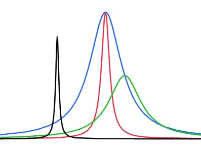
Gaussian Peak	a = Peak Value b = Critical Point c = Growth Rate
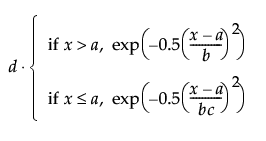
Asymmetric Gaussian Peak	a = Critical Value b = Scale 1 c = Scale 2 d = Peak Value Available only when the response values are nonnegative.
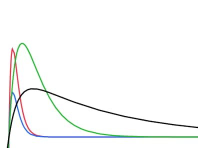
Skew Normal Peak	a = Location b = Scale c = Skew d = Peak Value φ = the standard normal pdf Available only when the response values are nonnegative.
ExGaussian Peak (Exponentially Modified Gaussian Peak)	a = AUC (area under the curve) b = Location c = Scale d = Lambda φ = the standard normal pdf
Pseudo-Voigt Peak	d = Mixing Parameter l(x) = evaluation of Lorentzian Peak function g(x) = evaluation of Gaussian Peak function Available only when the response values are nonnegative.
Pearson VII Peak	a = Location b = Scale c = Shape d = Peak Value Available only when the response values are nonnegative.
Lorentzian Peak	a = Peak Value b = Growth Rate c = Critical Point
One Compartment Oral Dose	a = Area Under Curve b = Elimination Rate c = Absorption Rate Available only when the response values and the x values are all positive.
Two Compartment IV Bolus Dose	α = β = a = Initial Concentration b = Transfer Rate In c = Transfer Rate Out d = Elimination Rate Available only when the response values and the x values are all positive.
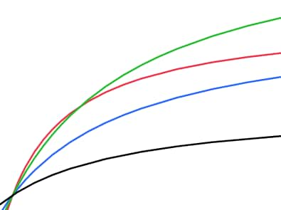
Michaelis-Menten	a = Maximum Velocity b = Michaelis Constant Available only when the response values and the x values are all positive.
Inverse Michaelis-Menten	a = Maximum Velocity b = Michaelis Constant Available only when the response values and the x values are all positive.
First Order Rate	a = Initial Value b = Rate Constant Available only if the x values are nonnegative.
First Order with Limits	a = Initial Value b = Limiting Value c = Rate Constant Available only if the x values are nonnegative.
First Order with Equilibrium	a = Initial Value b = Forward Rate c = Backward Rate Available only if the x values are nonnegative.
Second Order	a = Initial Value b = Rate Constant Available only if the x values are nonnegative.
Second Order with Two Components	a = Initial value b = Offset c = Rate Constant Available only if all x values are nonnegative.
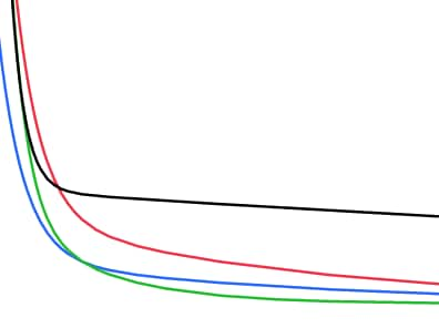
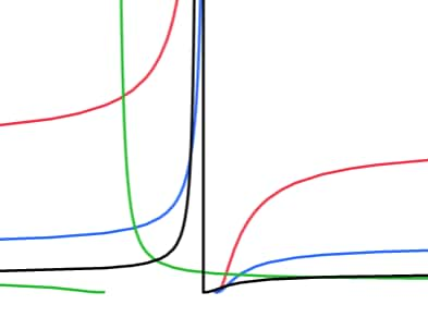
Antoine Equation	a = Component Specific Constant b = Component Specific Constant c = Component Specific Constant Available only when the response values are greater than 0. The vertical asymptote is at 10a. The horizontal asymptote is at −c.
Higuchi	a = Release Constant Available only if all x and y values are nonnegative.
Higuchi with Lag	a = Release Constant b = Time Lag Available only if all x and y values are nonnegative.
Higuchi with Burst	a = Release Constant b = Burst Available only if all x and y values are nonnegative.
Hixson-Crowell	a = Release Constant Available only if all x and y values are nonnegative.
Hixson-Crowell with Lag	a = Release Constant Available only if all x and y values are nonnegative.
Korsmeyer-Peppas	a = Release Constant b = Diffusional Exponent Available only if all x and y values are nonnegative.
Korsmeyer-Peppas with Lag	a = Release Constant b = Diffusional Exponent c = Time Lag Available only if all x and y values are nonnegative.
Korsmeyer-Peppas with Burst	a = Release Constant b = Diffusional Exponent c = Burst Available only if all x and y values are nonnegative.

Want more information? Have questions? Get answers in the JMP User Community (community.jmp.com).