Time to Event
The Time to Event panel in the Cumulative Damage launch window contains the following options:
Time to Event
Identifies the time to event (such as the time to failure) or time to censoring. For interval censoring, your data table should contain two columns, where one gives the lower bound and the other gives the upper bound of the failure time for each unit. Enter the two censoring columns as Time to Event. For more information about censoring, see Event Plot.
Censor
Identifies right-censored observations. Select the value that identifies right-censored observations from the Censor Code menu beneath the Select Columns list. The Censor column is used only when one Y is entered.
Freq
Identifies frequencies or observation counts when there are multiple units. If the value is 0 or a positive integer, then the value represents the frequencies or counts of observations with the given row’s settings.
Pattern ID
Contains values that specify the stress pattern in the Stress Pattern data table that was used for the given row.
Censor Code
Identifies the value in the Censor column that designates right-censored observations. After a Censor column is selected, JMP attempts to automatically detect the censor code and display it in the box. To change this, you can click the red triangle and select from a list of values. You can also enter a different value in the box. If the Censor column contains a Value Labels column property, the value labels appear in the list of values. Missing values are excluded from the analysis.
Relationship
Identifies the relationship between the event and the stress factor. Table 5.1 defines the model for each relationship.
|
Relationship |
Model |
|---|---|
|
Arrhenius Celsius |
μ = b0 + b1 * 11604.5181215503 / ( X + 273.15 ) |
|
Arrhenius Fahrenheit |
μ = b0 + b1 * 11604.5181215503 / ( ( X + 459.67 ) / 1.8 ) |
|
Arrhenius Kelvin |
μ = b0 + b1 * 11604.5181215503 / X |
|
Inverse Power (default) |
μ = b0 + b1 * log( X ) |
|
Linear |
μ = b0 + b1 * X |
|
Log |
μ = b0 + b1 * log( X ) |
|
Logit |
μ = b0 + b1 * log( X / ( 1 - X ) ) |
|
Reciprocal |
μ = b0 + b1 / X |
|
Square Root |
μ = b0 + b1 * sqrt( X ) |
|
Box-Cox |
μ = b0 + b1 * BoxCox( X ) |
|
Custom |
user-defined (Available only in the Step Stress panel.) |
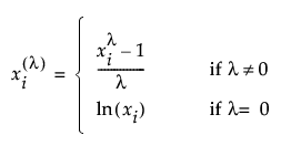
The BoxCox( X ) transformation is defined as follows:

If you select Custom, additional controls appear that require you to define the Custom transformation that models the relationship between the lifetime event and the stress factor.
If you want to use a Custom relationship for your model, see Custom Relationship.
Distribution
Specifies an initial time-to-failure distribution. Select from Weibull, Lognormal, Loglogistic, Fréchet, or Exponential. Weibull is the default setting. For more information about the distributions, see Statistical Details for Distributions.