Example of Comparing Multiple Latent Growth Curve Models
Latent Growth Curve (LGC) models offer a flexible approach for investigating how processes change over time. You can define and compare different trajectories, including no-growth, linear, quadratic, and non-linear trajectory using the Latent Basis Growth Curve option in the Model Shortcuts menu. The Fit and Compare Growth Models option in the Model Shortcuts menu enables you to specify, fit, and compare growth curve models simultaneously. In this example, you are modeling achievement scores of students over 4 years of an academic program using a multiple choice test score. You want to compare different growth patterns to see which trajectory best characterizes this process.
1. Select Help > Sample Data Folder and open Academic Achievement.jmp.
2. Select Analyze > Multivariate Methods > Structural Equation Models.
3. Select Multiple Choice Year1 through Multiple Choice Year4 and click Model Variables.
4. Click OK.
5. Select Model Shortcuts > Longitudinal Analysis > Fit and Compare Growth Models.
The Model Specification diagram now shows a quadratic latent growth curve model.
The Structural Equation Models report that appears includes two parts. The first part contains the Model Specification, Model Comparison, and Chi-Square Difference Test reports. The Model Comparison and Chi-Square Difference Test reports can be used to compare all fitted growth models in one place. Specifically, the Chi-Square Difference Test report can help determine whether a more complex model significantly improves the fit to the data compared to a simpler model that is nested within the more complex model.
The second part of the Structural Equation Models report contains model reports that include a Summary of Fit report, a Parameter Estimates report, and a Path Diagram for each of the specified models. The individual model reports can be used to evaluate how well each model fits the data.
Figure 8.13 Model Comparison and Chi-Square Difference Test Reports
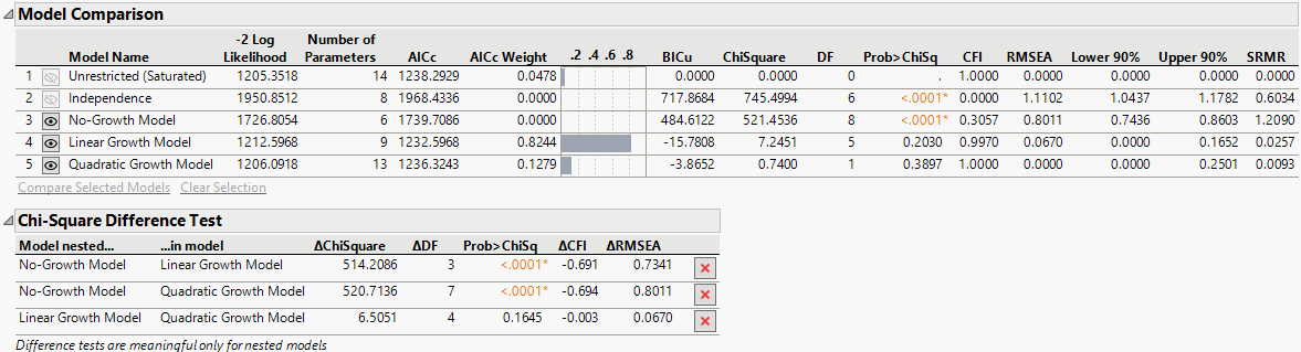
The Model Comparison report in Figure 8.13 contains fit indices for five models: the Unrestricted (Saturated), the Independence, the No-Growth, the Linear Growth, and the Quadratic Growth models. Overall, the Linear Growth model is the most supported model compared to other models. This conclusion is based on the largest AICc Weight value (0.82) and very good fit indices (CFI = 0.997, RMSEA = 0.067). The Quadratic Growth model also fits the data well, with perfect fit indices (CFI = 1 and RMSEA = 0), but it is less favored based on the AICc Weight. The Independence and No-Growth models show poor fits, with high ChiSquare values and inadequate fit indices, which indicate that they do not represent the data well.
Note: It is important to select the appropriate independence model when comparing growth models. The No-Growth model is typically recommended as the independence model because it serves as a meaningful baseline to evaluate the fit of other growth trajectories. However, you can choose any other trajectory as the independence model. To do this, select a row in the Model Comparison report, right-click, and select the Set as Independence Model option. To revert to the default independence model, right-click on the selected model and choose the Reset Default Independence Model option.
The Chi-Square Difference Test report shown in Figure 8.13 also compares the fit of these models. The comparisons are made by looking at changes in the chi-square statistic, CFI, and RMSEA between the nested models. Overall, it can be concluded from this report that the No-Growth model fits significantly worse than both the Linear and Quadratic Growth models. There is no significant difference between the Linear and Quadratic Growth models, which suggests that adding a quadratic term does not significantly improve the model fit over the linear model. While the Quadratic Growth model fits the data very well, the marginal improvement in fit does not justify its additional complexity over the Linear Growth model. Therefore, the Linear Growth model is likely the best choice as it offers a good fit without the added complexity of the Quadratic Growth model.
Next, consider the Model Comparison and Chi-Square Difference Test reports together. Since the Linear Growth model is the most supported model with the highest AICc weight (0.82) and demonstrates excellent fit indices (CFI = 0.997, RMSEA = 0.07), it should be considered the most appropriate model. Also, the nested comparisons indicate that while the Quadratic Growth model results in a slightly improved fit, the difference with the Linear Growth model is not statistically significant. Thus, the Linear Growth model offers a good balance between simplicity and model fit. There is strong evidence from the nested model comparison that the Linear Growth model provides a significantly better fit than the No-Growth model.
You can also check fit indices and compare models using the model reports that are generated for each of the specified models. The Linear Growth model appears to be well-specified and fits the data well. The model converged quickly with a small number of parameters, and the fit indices are well within acceptable ranges, which indicates a strong fit. The Quadratic Growth model has some fit indices that suggest a good model, but these apparent strengths are overshadowed by serious issues, which include a negative variance estimate and a nonpositive definite covariance matrix. The intercept and linear slope are significantly different from zero, which suggests a significant initial level and a linear growth trend over time. However, the quadratic slope is not significant, which suggests that the quadratic component may not be necessary.
Both parts of the Structural Equation Models report indicate that the Linear Growth model appears to be well-specified and fits the data well. It captures both the initial levels and the linear trends over time and accounts for individual differences in both intercepts and slopes.