Defect Profiler
From the Simulator red triangle menu, you can launch the Defect Profiler. This profiler shows the probability of an out-of-spec output defect as a function of each factor while the other factors vary randomly. This is used to help visualize the changes in a factor’s distribution that the process is most sensitive to, often as part of tolerance design.
Specification limits are used to define a defect, and the random distributions assigned to each factor are used to simulate responses. To use the Defect Profiler, specification limits must be defined for at least one response.
Define at least one of the factors as Random in the simulation settings to obtain useful results. Otherwise, the simulation outputs are constant and the defect rate is zero if the outcome falls within spec or one if the outcome falls out of spec.
Tip: If you need to estimate very small defect rates, consider the Normal weighted random option. This random distribution estimates stable defect rates of just a few parts per million with only a few thousand simulation runs.
Introduction to Tolerance Design
Tolerance design is the investigation of how defect rates can be controlled by controlling variability in the input factors.
Input factors have variation. Specification limits are used to define acceptable ranges for each input. The variability in the input factors impacts the outputs. Specification limits are also used to define the acceptable range for output variables.
Sometimes, a tolerance design study shows that spec limits on an input are unnecessarily tight. Loosening such limits can result in reduced costs without sacrificing product quality. In these cases, tolerance design can save money.
In other cases, a tolerance design study might find that either tighter limits or different targets result in higher quality. In all cases, it is valuable to understand how the inputs and their variability impact that the defect rates.
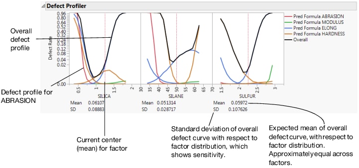
The Defect Profiler shows the defect rate as a function of each factor fixed at the specified mean value while all other factors are varied according to their random specification. If there are multiple outputs with spec limits, each has a different colored defect rate curve. A black curve shows the overall defect rate.
Figure 8.7 Defect Profiler
Graph Scale
Defect rates are shown on a cubic root scale, so that both large and small defect rates are shown in some detail.
Defect Rates
The mean and standard deviation (SD) of the simulated overall defect rate are reported below each defect profile plot. This mean is calculated by integrating the defect profile curve with the specified factor distribution. Because of numerical error in the estimations, the overall mean defect rate reported under each factor can differ slightly.
The defect rates that are reported in the Defect Profiler are estimates of the simulated overall defect rate. This rate is also reported in the Rate column of the defect table that is in the Prediction Profiler outline.
Note: The defect table is added to the Prediction Profiler outline after you run a simulation and one or more of your responses has defined spec limits.
Because the rate estimates are obtained differently, by integration and simulation, they might differ slightly. If they are very different, you might consider increasing the number of simulation runs. In addition, verify that the range of the factor scale is wide enough so that the integration covers the distribution well.
The standard deviation is a measure of the sensitivity of the defect rate to the factor. It is small when either the factor profile is flat or the factor distribution has a small variance. The larger the standard deviation, the larger the impact that changes in that factor have on the defect rate variability. Comparing SDs across factors enables you to select factors for improvement to reduce defect rates.
The mean and SD values are updated when you change the factor distribution settings. This is one way to explore how to reduce defects as a function of one particular factor at a time. You can click and drag a handle point on the factor distribution and watch the mean and SD change as you drag. However, changes are not updated across all factors until you click the Rerun button to generate updated simulation runs.
Simulation Method and Details
Suppose you want a defect profile for factor X1, in the presence of random variation in X2 and X3. A series of n = N Runs simulation runs is done at each of k points in a grid of equally spaced values of X1. (By default, k is set at 17.) At each grid point, suppose that there are m defects due to the specification limits. At that grid point, the defect rate is m/n. These defect rates are connected and plotted as a continuous function of X1.
Notes
• The profile curve is not recalculated automatically when distributions change. Click Rerun to update the curve.
• Defect Profiling does not address the general optimization problem of optimizing quality against cost, given functions that represent all aspects of the problem. This more general problem would benefit from a surrogate model and space filling design.
• The defect profiles tend to be uneven when they are low. This is due, in part, to the use of the cubic scale where differences in low values are exaggerated. Jagged defect profiles could be due to limited simulation runs. If the overall defect curve (black line) is smooth, and the individual defect rates are fairly consistent, then your simulation probably has enough runs to provide a stable solution. If the overall defect rate curve is jagged, then consider increasing the number of runs. 20,000 runs is generally enough to stabilize the curves.
