Example of the Surface Plot
In this example, you use prediction formula columns to examine the surfaces of two response variables.
1. Select Help > Sample Data Folder and open Tiretread.jmp.
2. Select Graph > Surface Plot.
3. Select Pred Formula ABRASION and Pred Formula MODULUS, click Columns, and then click OK.
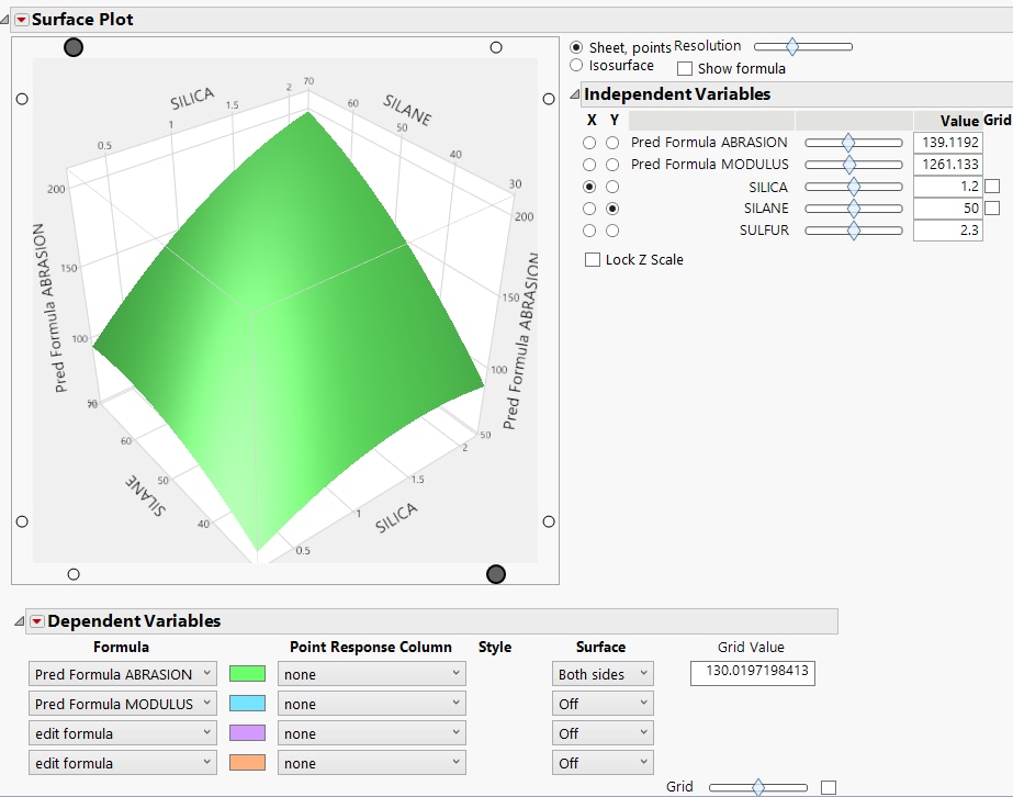
Figure 5.2 Initial Surface Plot Report
Initially, only the prediction surface for ABRASION appears in the plot. Note that in the Independent Variables report, there is a large difference between the values for ABRASION and MODULUS. The two responses are on different scales.
4. In the Dependent Variables report, select Both Sides from the Surface list for Pred Formula MODULUS.
5. Click the Surface Plot red triangle and select Scale response axes independently.
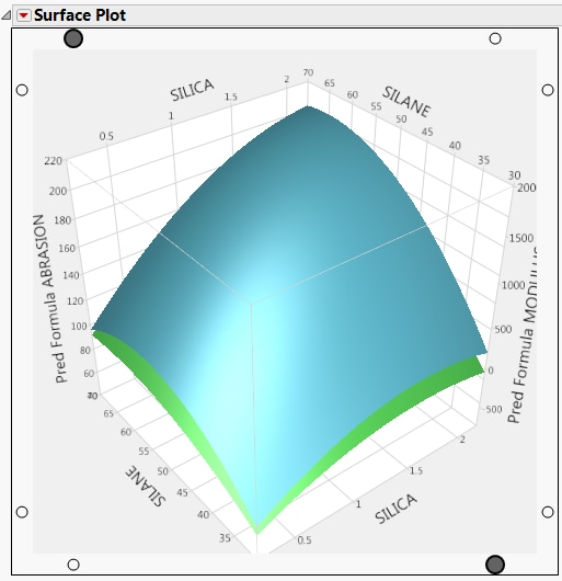
Figure 5.3 Prediction Surface for ABRASION and MODULUS
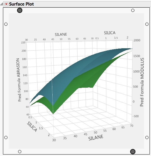
Pred Formula ABRASON is on one Z axis and Pred Formula MODULUS is on the other Z axis. Each response has its own scale. In this plot, the two factors considered are SILICA and SILANE. You can rotate the surface plot by clicking and dragging inside the graph. This enables you to view the prediction surfaces from different perspectives. For example, in Figure 5.4, you can see that predictions for ABRASION and MODULUS based on the two listed predictors have a similar surface shape, just on a different scale. Use the Independent Variables controls to see how different combinations of predictors affect the surface plot.
Tip: To see the original view after rotating, right-click anywhere on the surface plot and select Reset.
Figure 5.4 Rotated Prediction Surfaces


