Example of Accelerated Destructive Degradation
This example fits a custom nonlinear model in the Degradation platform. The data consist of measurements on the strength of an adhesive bond. The product is stressed until the bond breaks, and the required breaking strength is recorded. Because units at normal use conditions are unlikely to break, the units were tested at several levels of an acceleration factor (temperature). You want to estimate the strength (in newtons) of units after 52 weeks (one year) at use conditions of 25oC.
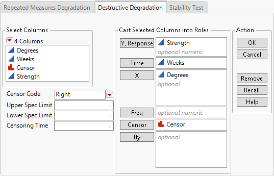
Complete the Launch Window
1. Select Help > Sample Data Folder and open Reliability/Adhesive Bond.jmp.
2. Select Analyze > Reliability and Survival > Degradation.
3. Select the Destructive Degradation tab.
4. Select Strength and click Y, Response.
5. Select Weeks and click Time.
6. Select Degrees and click X.
7. Select Censor and click Censor.
Figure 16.21 Completed Launch Window
8. Click OK.
Define and Fit the Model
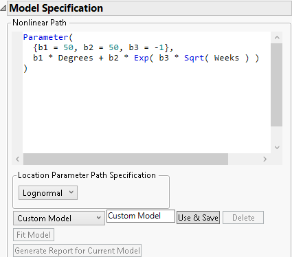
1. Select Lognormal from the menu in the Location Parameter Path Specification panel in the Model Specification outline.
This specifies a lognormal transformation for the response, Strength.
2. Click the Degradation Data Analysis red triangle and select Degradation Path Style > Nonlinear Path.
This adds a script window to the report. You insert a script that specifies your model in this window.
3. Copy the JSL formula below and paste it into the script window under Nonlinear Path:
Parameter( {b1 = 50, b2 = 50, b3 = -1}, b1 * :Degrees + b2 * Exp( b3 * Sqrt( :Weeks ) ))The script defines a model for Strength in terms of parameters b1, b2, and b3. The script specifies initial values for the parameters.
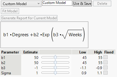
4. In the text box at the bottom of the report, change Empty to Custom Model.
Figure 16.22 Nonlinear Path Script
5. Click Use & Save.
Figure 16.23 Updated Model Specification Outline
The report is updated to include controls for changing initial values for the parameters. Initial values for the parameters are set to the values specified in the formula in the script editor.
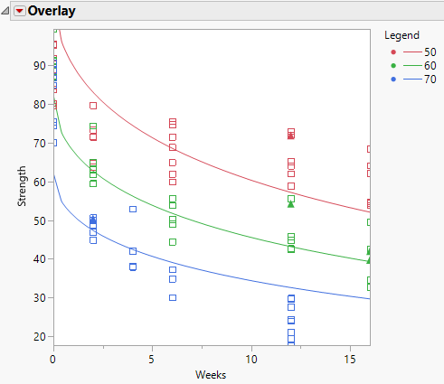
6. Click Fit Model.
Figure 16.24 Plot of Fitted Model
The Parameter panel in the Model Specification outline is updated to show the parameter estimates for the fitted model. The model fit is shown in the Overlay plot. You can drag the axes to show the points, as is done in Figure 16.24. The legend identifies the curves.
Obtain Predicted Values and Prediction Intervals
Next, you obtain a predicted value and prediction interval for Strength after 52 weeks at the baseline use condition of 25oC.
1. Click the Degradation Data Analysis red triangle and select Prediction Settings.
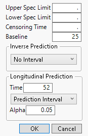
2. In the Prediction Settings window:
– Enter 25 for Baseline.
– Enter 52 for Time in the Longitudinal Prediction panel.
– Select Prediction Interval from the menu in the Longitudinal Prediction panel.
Figure 16.25 Prediction Settings
3. Click OK.
4. Select the Prediction Graph tab in the report.
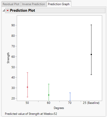
Figure 16.26 Prediction Plot at Weeks = 52
The Prediction Plot shows the predicted value and its 95% level prediction interval above the axis label of 25 (Baseline).
5. Click the Prediction Plot red triangle and select Save Predictions.
Predicted values for the three values of Degrees and for the desired baseline of 25 degrees are saved to a data table. The predicted strength of the adhesive bond after 1 year at 25o C is 61.96, with a prediction interval of 42.42 to 90.50.
