Example of Inverse Prediction
Use the Standard Least Squares personality of the Fit Model platform to fit a linear regression model and then obtain predictions of the input based on specified response levels. This is known as an inverse prediction. This example considers one predictor. For multiple predictors, see Example of Inverse Prediction for Multiple Predictors.
1. Select Help > Sample Data Folder and open Fitness.jmp.
2. Select Analyze > Fit Model.
3. Select Oxy and click Y.
4. Select Runtime and then click Add.
5. Click Run.
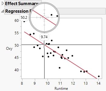
Use the crosshairs tool as described below to approximate the Runtime value that results in a mean Oxy value of 50 from the Regression Plot.
6. Select Tools > Crosshairs.
7. Click on the prediction line and then drag the crosshairs tool to find the inverse prediction for Oxy = 50.
Figure 4.50 Regression Plot Oxy as a Function of Runtime
From the Regression Plot, you estimate that the inverse prediction of an Oxy value of about 50 is a Runtime of about 9.7
To obtain an exact inverse prediction and confidence interval for Runtime, continue with the steps below:
8. Click the Response Oxy red triangle and select Estimates > Inverse Prediction.
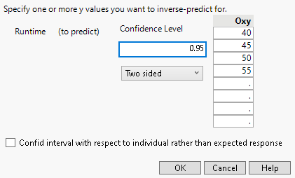
Enter four values for Oxy as shown in Figure 4.51.
9. Click OK.
Figure 4.51 Completed Inverse Prediction Specification Window
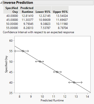
The Inverse Prediction report gives predicted Runtime values that correspond to each specified Oxy value. The report also shows upper and lower 95% confidence limits for these Runtime values, relative to obtaining the mean response.
Figure 4.52 Inverse Prediction Report
The predicted Runtime resulting in an Oxy value of 50 is 9.7935. This value is close to the approximate Runtime value of 9.7 found using the Regression Plot. The Inverse Prediction report also gives a plot showing the linear relationship between Oxy and Runtime and the inverse prediction confidence intervals.


