 Launch the Generalized Linear Mixed Model Personality
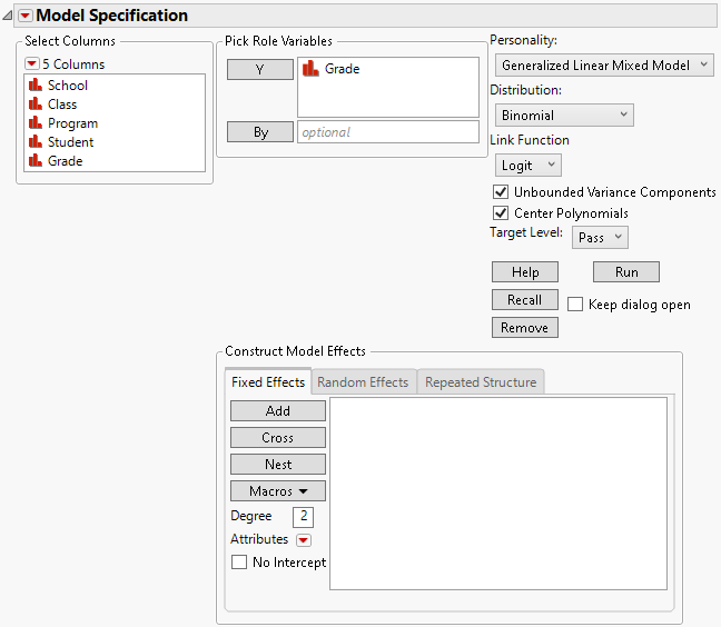
Launch the Generalized Linear Mixed Model personality by selecting Analyze > Fit Model, entering one or more columns for Y, and selecting Generalized Linear Mixed Model from the Personality menu.
 Fit Model Launch Window
You can specify models with fixed effects, random effects, or a combination of fixed and random effects. You can also specify a distribution for the response variable. The options in the launch window differ based on the nature of the model that you specify. For more information about the options in the Select Columns red triangle menu, see “Column Filter Menu” in Using JMP.
When fitting models using the Generalized Linear Mixed Model personality, you can allow unbounded variance components. This means that variance components that have negative estimates are not reported as zero. This option is selected by default. It should remain selected if you are interested in fixed effects, because bounding the variance estimates at zero leads to bias in the tests for fixed effects. See “Negative Variances” for more information about the Unbounded Variance Components option.
Figure 9.6 Fit Model Launch Window with Generalized Linear Mixed Model Selected
For more information about aspects of the Fit Model window that are common to all personalities, see “Model Specification”. For more information about the options in the Select Columns red triangle menu, see “Column Filter Menu” in Using JMP. Information specific to the Generalized Linear Mixed Model personality is presented here.
 Specify a Distribution
In the Fit Model launch window, when you select Generalized Linear Mixed Model as the Personality, the Distribution option appears. Here you can specify a distribution for Y. The available distributions are described below.
Normal
Specifies that Y has a normal distribution with mean μ and standard deviation σ. The normal distribution is symmetric and with a large enough sample size, can approximate a large variety of other distributions using the Central Limit Theorem. The link function for μ is the identity, which implies that the mean of Y is expressed as a linear model.
Exponential
Specifies that Y has an exponential distribution with mean parameter μ. The exponential distribution is right-skewed and is often used to model lifetimes or the time between successive events. The link function for μ is the logarithm.
Gamma
Specifies that Y has a gamma distribution with mean parameter μ and dispersion parameter σ. The gamma is a flexible distribution and contains a family of other widely used distributions. For example, the exponential distribution is a special case of the gamma distribution where σ = μ. The chi-squared distribution can also be derived from the gamma distribution. The link function for μ is the logarithm.
LogNormal
Specifies that Y has a lognormal distribution with location parameter μ and scale parameter σ. The lognormal distribution is right-skewed and is often used to model lifetimes or the time until an event. The link function for μ is the identity.
Beta
Specifies that Y has a beta distribution with mean parameter μ and dispersion parameter σ. The response for the beta is between 0 and 1 (not inclusive) and is often used to model proportions or rates. The link function for μ is the logit.
Binomial
Specifies that Y has a binomial distribution with parameters p and n. The response, Y, indicates the total number of successes in n independent trials with a fixed probability, p, for all trials. This distribution allows for the use of a sample size column. If no column is listed, it is assumed that the sample size is one. By default, the link function for p is the logit. You can change the link function for p to the probit using the Link Function option in the Fit Model launch window. When you select a binary response variable that has a Nominal modeling type, Binomial is the only available response distribution.
When you select Binomial as the Distribution, the response variable must be specified in one of the following ways.
– Unsummarized: If your data are not summarized as frequencies of events, specify a single binary column as the response. If this column has a modeling type of Nominal, you can designate one of the levels to be the Target Level. The default Target Level value is the higher of the two levels based on the order of the levels.
– Summarized with sample size column entered as second Y: If your data are summarized as frequencies of events (successes) and trials, specify two continuous columns as Y in this order: the count of the number of successes, and the count of the number of trials.
Poisson
Specifies that Y has a Poisson distribution with mean λ. The Poisson distribution typically models the number of events in a given interval and is often expressed as count data. The link function for λ is the logarithm. Poisson regression is permitted even if Y assumes noninteger values.
Negative Binomial
Specifies that Y has a negative binomial distribution with mean μ and dispersion parameter σ. The negative binomial distribution typically models the number of successes before a specified number of failures. The negative binomial distribution is also equivalent to the Gamma Poisson distribution under certain conditions. For more information about the connection between negative binomial and Gamma Poisson, see “Distributions” in Basic Analysis.
Run demoGammaPoisson.jsl in the JMP Samples/Scripts folder to compare a Gamma Poisson distribution with mean λ and dispersion parameter σ to a Poisson distribution with mean λ.
The link function for μ is the logarithm. Negative binomial regression is permitted even if Y assumes noninteger values.
The following table provides the Data Types, Modeling Types, and other requirements for Y variables that are assigned the various distributions.
Distribution | Data Type | Modeling Type | Other |
|---|---|---|---|
Normal | Numeric | Continuous |
|
Exponential | Numeric | Continuous | Nonnegative |
Gamma | Numeric | Continuous | Positive |
LogNormal | Numeric | Continuous | Positive |
Beta | Numeric | Continuous | Between 0 and 1 |
Binomial, unsummarized | Any | Any | Binary |
Binomial, summarized with count column entered as second Y | Numeric | Continuous | Nonnegative |
Poisson | Numeric | Any | Nonnegative |
Negative Binomial | Numeric | Any | Nonnegative |
The following table provides a summary of the distribution parameterization and link functions.
Distribution | Parameters | Mean Model Link Function |
|---|---|---|
Normal | μ, σ | Identity(μ) |
Exponential | μ | Log(μ) |
Gamma | μ, σ | Log(μ) |
LogNormal | μ, σ | Identity(μ) |
Beta | μ | Logit(μ) |
Binomial | n, p | Logit(p) Probit(p) |
Poisson | λ | Log(μ) |
Negative Binomial | μ, σ | Log(μ) |
 Fixed Effects Tab
Add all fixed effects on the Fixed Effects tab. Use the Add, Cross, Nest, Macros, and Attributes options as needed. For more information about these options, see “Model Specification”. Note that it is possible to have no fixed effects in the model.
Note: If a continuous column is involved in a random effect, that column is not centered, even if the Center Polynomials option in the Model Specifications red triangle menu is selected.
Figure 9.7 Completed Fit Model Launch Window Showing Fixed Effects
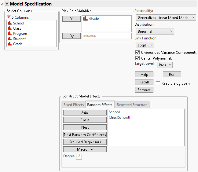
 Random Effects Tab
Specify traditional variance component models and random coefficients models using the Random Effects tab.
Note: If a continuous column is involved in a random effect, that column is not centered, even if the Center Polynomials option in the Model Specifications red triangle menu is selected.
Variance Components
For a traditional variance component model, specify terms such as random blocks, whole plot error terms, and subplot error terms using the Add, Cross, or Nest options. For more information about these options, see “Model Specification”.
Figure 9.8 Completed Fit Model Launch Window Showing Random Effects
Random Coefficients
To construct random coefficients models, use the Nest Random Coefficients button to create groups of random coefficients.
1. Select the continuous columns from the Select Columns list that are predictors.
2. Select the Random Effects tab and then Add.
3. Select these effects in the Random Effects tab. Also select the column that contains the random effect whose levels define the individual regression models.
4. Click the Nest Random Coefficients button.
This last step creates random intercept and random slope effects that are correlated within the levels of the random effect. The subject is nested within the other effects due to the variability among subjects. If you believed that the intercept might be fixed for all groups, you would select Intercept[<group>]&Random Coefficients(1) and then click Remove.
You can define multiple groups of random coefficients in this fashion, as in hierarchical linear models. This might be necessary when you have both a random batch effect and a random batch by treatment effect on the slope and intercept coefficients. This might also be necessary in a hierarchical linear model: when you have a random student effect and random school effect on achievement scores and students are nested within school.
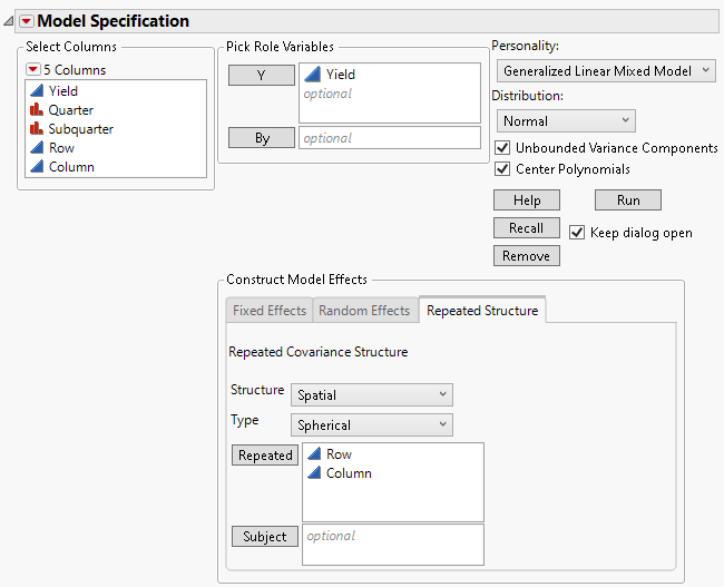
 Repeated Structure Tab
Use the Repeated Structure tab to select a covariance structure for repeated effects in the model.
Table 9.3 Completed Fit Model Launch Window Showing Repeated Structure Tab

Structure
The repeated structure is set to None by default. The None structure specifies that there is no covariance between observations, namely, the errors are independent. All other covariance structures model covariance between observations.
Table 9.4 lists the covariance structures that are available, the requirements for using each structure, and the number of covariance parameters for the given structure. The number of observation times is denoted by J.
Structure | Repeated Column Type | Required Number of Repeated Columns | Subject | Number of Parameters |
|---|---|---|---|---|
None | not applicable | 0 | not applicable | 0 |
Unstructured | categorical | 1 | required | J(J+1)/2 |
AR(1) | continuous | 1 | optional | 2 |
Compound Symmetry | categorical | 1 | required | 2 |
Toeplitz | categorical | 1 | required | J |
Antedependent | categorical |
| required | 2J-1 |
Spatial | continuous | 2+ | optional |
|
If you enter a Repeated or Subject column with the None structure, those columns are ignored. This alert appears: “Repeated columns and subject columns are ignored when the Residual covariance structure is selected.”
Type
When you select the Spatial covariance structure, a Type list appears from which you select a type of spatial structure. Four Types are available: Power, Exponential, Gaussian, and Spherical.
Repeated
Enter columns that define the repeated measures structure. The modeling types of Repeated columns depend on the covariance structure. See Table 9.4 for more information about the requirements for each repeated measures covariance structure.
Subject
Enter one or more columns that define the Subject. Subject columns must be categorical.
 Data Format
The Generalized Linear Mixed Model personality of the Fit Model platform requires that all response measurements be contained in one response column. Repeated measures data are sometimes recorded in multiple columns, where each row is a subject and the repeated measurements are recorded in separate response columns. Data that are in this format must be stacked before running the Generalized Linear Mixed Model personality. The Cholesterol.jmp and Cholesterol Stacked.jmp sample data tables illustrate the wide format and the stacked format, respectively. Notice that each row in the wide table corresponds to one level of Patient in the stacked table.


