 Example of Bagging to Indicate the Accuracy of Predictions
Bagging is also used to indicate the accuracy of the prediction through standard errors and other distributional measures. In platforms where the Save Predicted Formulas option is available in Bagging, you can make predictions on new observations and determine how accurate they are. The Save Predicted Formulas option is available in the Standard Least Squares, Generalized Regression, and Generalized Linear Models platforms.
In the Tiretread.jmp data table, suppose that you are interested in only predicting ABRASION as a function of the three factor variables. In this example, you fit a generalized regression model to predict ABRASION. Then, you perform bagging on that model. Last, you make a prediction for a new observation and investigate the accuracy of that prediction. This is done by obtaining a confidence interval for the prediction.
Fit a Generalized Regression Model
1. Select Help > Sample Data Folder and open Tiretread.jmp.
2. Select Analyze > Fit Model.
3. Select ABRASION and click Y.
4. Select Generalized Regression from the Personality list.
5. Select SILICA, SILANE, and SULFUR and click Macros > Full Factorial.
This adds all terms, including interactions, to the model.
6. Click Run.
7. Click Go.
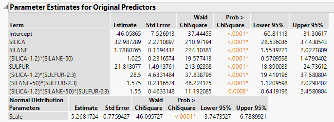
Figure 3.35 Parameter Estimates From Generalized Regression Report
Perform Bagging
1. Click the red triangle next to Normal Lasso with AICc Validation and select Profilers > Profiler.
The Prediction Profiler appears at the bottom of the report.
2. Click the Prediction Profiler red triangle and select Save Bagged Predictions.
3. Enter 500 next to Number of Bootstrap Samples.
4. (Optional) Enter 4321 next to Random Seed.
Note: Results vary due to the random nature of sampling with replacement. To reproduce the exact results in this example, set the Random Seed.
5. Confirm that Save Prediction Formulas is selected.
6. Click OK.
Note: This might take longer to run than the Example of Bagging to Improve Prediction. The larger number of samples gives a better estimate of the prediction distributions.
Return to the data table. For each response variable, there are three new columns denoted as Pred Formula <colname> Bagged Mean, <colname> Bootstrap Std Err, and StdError <colname> Bagged Mean. The Pred Formula ABRASION Bagged Mean column is the final prediction.
Prediction for a New Observation
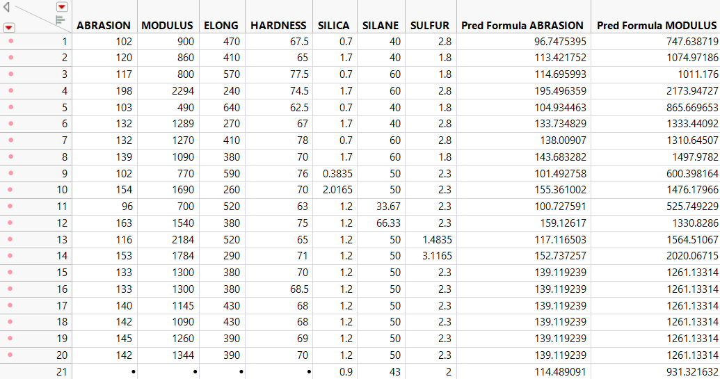
You now have predictions for ABRASION for each observation in the data table, as well as the standard errors for those predictions. Suppose that you have an observation with new values of 0.9, 43, and 2 for SILICA, SILANE, and SULFUR, respectively. You can predict the ABRASION response and obtain a confidence interval for that prediction because the Save Prediction Formulas option saves the regression equation for each bagged model. Therefore, M predictions are made with the new factor values to create a distribution of possible predictions. The mean is the final prediction, but analyzing the distribution tells you how accurate the prediction is.
1. In the data table, select Rows > Add Rows.
2. Enter 1 in the How many rows to add box and click OK.
3. Under the SILICA column, type 0.9 in the box for the new row.
4. Under the SILANE column, type 43 in the box for the new row.
5. Under the SULFUR column, type 2 in the box for the new row.
All of the prediction columns for the new row are automatically calculated.
Figure 3.36 Values for New Row
6. Select Tables > Transpose.
7. Select ABRASION Bags (500/0) and click Transpose Columns.
8. Click OK.
9. Select Analyze > Distribution.
10. Select Row 21 and click Y, Columns.
Note: Row 21 corresponds to the predictions from the new observation.
11. Click OK.
12. Click the red triangle next to Row 21 and select Display Options > Horizontal Layout.
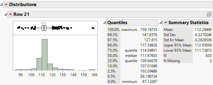
Figure 3.37 Distribution Report
The Distribution Report in Figure 3.37 contains information about the distribution of the predicted values of ABRASION from each bagged model. The final prediction of ABRASION for the new observation is 112.3, which is the mean of all the M bagged predictions. This prediction has a standard error of 6.33. You can also create confidence intervals for the new prediction using the quantiles. For example, a 95% confidence interval for the new prediction is 102.09 to 127.62.


