Time Series Models

The Time Series red triangle menu contains options to fit the following types of models.

ARIMA

Shows the ARIMA Specification window, which enables you to specify the ARIMA model that you want to fit. An ARIMA model predicts future values of a time series by a linear combination of its past values and a series of errors (also known as random shocks or innovations). The ARIMA model performs a maximum likelihood fit of the specified ARIMA model to the time series. See ARIMA Model.

Note: An ARIMA model is commonly denoted ARIMA(p,d,q). If any of p, d, or q are zero, the corresponding letters are often dropped. For example, if p and d are zero, then the model would simply be a moving average model, denoted as MA(q).

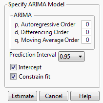
Figure 18.6 ARIMA Specification Window 

p, Autoregressive Order

The order p of the polynomial ϕ(B) operator.

d, Differencing Order

The order d of the differencing operator.

q, Moving Average Order

The order q of the differencing operator θ(B).

Prediction Interval

Enables you to set the prediction level between 0 and 1 for the forecast prediction intervals.

Intercept

Determines whether the intercept term μ is a part of the model.

Constrain fit

If checked, the fitting procedure constrains the autoregressive parameters to always remain within the stable region and the moving average parameters within the invertible region.

Tip: Deselect the Constrain fit option if the fitter is having difficulty finding the true optimum or if you want to speed up the fit. You can use the Model Summary table to see whether the resulting fitted model is stable and invertible.

Once you specify the model and click Estimate, a Model Report is added to the report window. See Additional Time Series Reports.

Seasonal ARIMA

Shows the Seasonal ARIMA Specification window, which enables you to specify the Seasonal ARIMA model that you want to fit. This window has the same elements as the ARIMA specification window, but it also contains the seasonal element specifications. The additional Observations per Period option enables you to specify the number of observations per period, denoted as s. For more information about the Seasonal ARIMA model, see Seasonal ARIMA Model.

Note: Seasonal ARIMA models are denoted as Seasonal ARIMA(p,d,q)(P,D,Q)s.

Once you specify the model and click Estimate, a Model Report is added to the report window. See Additional Time Series Reports.

Smoothing Models

Shows a submenu of smoothing models. Once you select a smoothing model, a specification window appears. See Simple Smoothing Average Specification Window and Smoothing Model Windows. For each model that is specified, a Smoothing Model Report appears in the report window. See Model Report. Smoothing models represent the evolution of a time series by the model:

where

μt is the time-varying mean term

βt is the time-varying slope term

s(t) is one of the s time-varying seasonal terms

at are the random shocks

For more information about the general smoothing model equation, see Statistical Details for Exponential Smoothing Models. The following smoothing models are available:

Simple Moving Average

(Not available when either Forecast on Holdback or Use Box-Cox Transformation are selected in the launch window.) A model that estimates values by using an average of several adjacent points, defined by the smoothing window. The Simple Smoothing Average Specification window enables you to specify aspects of the smoothing window. Once the smoothing window options are specified, a Simple Moving Average report is shown. By default, this report produces plotted values that are equal to the average of consecutive observations in a time window. Multiple Simple Moving Average models can be added and shown on the same plot. See Simple Smoothing Average Specification Window.

Simple Exponential Smoothing

A model with a level component. See Simple Exponential Smoothing.

Double Exponential Smoothing

A model with a level component and a trend component. This is a special case of Linear Exponential Smoothing. See Double (Brown) Exponential Smoothing.

Linear Exponential Smoothing

A model with a level component and a trend component. See Linear (Holt) Exponential Smoothing.

Damped-Trend Linear Exponential Smoothing

A model with a level component and a damped trend component. This model is appropriate for a series that exhibits a trend more complicated than a linear trend. See Damped-Trend Linear Exponential Smoothing.

Seasonal Exponential Smoothing

A model with a level component and a seasonal component. See Seasonal Exponential Smoothing.

Winters Method

A model with a level component, a trend component, and a seasonal component. See Winters Method (Additive).

Note: Each smoothing model, except for the Simple Moving Average model, is a traditional exponential smoothing model and has an ARIMA model equivalent. You might not be able to specify the equivalent ARIMA model using the ARIMA option because some smoothing models intrinsically constrain the ARIMA model parameters in ways that the ARIMA option does not allow.

State Space Smoothing Models

Shows the Specify State Space Smoothing Models window, which enables you to fit a variety of state space smoothing models as defined by Hyndman et al. (2008). A state space smoothing model is defined based on its error, trend component, and seasonal component.

– The errors can be additive (A) or multiplicative (M).

– The trend component can be none (N), additive (A), additive damped (Ad), multiplicative (M), or multiplicative damped (Md).

– The seasonal component can be none (N), additive (A), or multiplicative (M).

A specific model can be represented by its ETS (Error, Trend, Seasonal). Use the check boxes in the Specify State Space Smoothing Models window to select the error, trend, and seasonality for the desired models. Click Select Recommended to select the check boxes that correspond to the models recommended by the platform. The window opens with the recommended models selected. Click Select All to select all check boxes or Deselect All to deselect all check boxes.

The window also contains the following options:

Period

Specifies seasonality values to be considered in the model fitting process.

Constrain Parameters

Constrains the parameters in such a way that the further an observation is from the present, the less effect that it has on the present state of the model. In State Space Smoothing models, a forecast at time t, given all previous observations, is the same as the weighted sum of all observations up to time t. The weights are a function of the parameters. Therefore, constraining the parameters ensures that the weights for past observations go to zero and that the further an observation is from the present, the faster the weight goes to zero.

When you click OK, the specified set of models is fit. Each State Space Smoothing model that is fit is added to the Model Comparison table. If the Report check box for a state space smoothing model in the Model Comparison table is selected, a State Space Smoothing report appears. See State Space Smoothing Report.

Transfer Function

(Available only in the Transfer Function Analysis red triangle menu.) Shows the Transfer Function Model Specification window. Building a transfer function model is similar to building an ARIMA model; it is an iterative process of exploring, fitting, and comparing models. Before building a model and during the data exploration process, it is sometimes useful to prewhiten the data. See Prewhitening. For more information about transfer functions, see Statistical Details for Transfer Functions.

Note: Currently, the Transfer Function option has limited support of missing values. Because the Time Series platform also treats excluded rows as missing values, transfer function models cannot be fit on a data table with excluded rows.

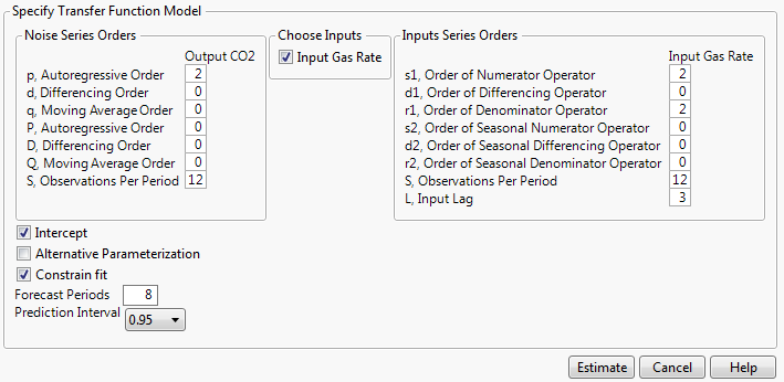
Figure 18.7 Transfer Function Model Specification Window 

The Transfer Function Model Specification window contains the following sections:

Noise Series Orders

Contains specifications for the noise series. Lowercase letters are coefficients for non-seasonal polynomials, and uppercase letters are coefficients for seasonal polynomials.

Choose Inputs

Enables you select the input series for the model.

Input Series Orders

Contains specifications for the input series. The first three orders relate to non-seasonal polynomials. The next four orders relate to seasonal polynomials. The final option is for an input lag.

There are three additional options that control model fitting:

Intercept

Specifies whether the model has an intercept. If unchecked, it is assumed that μ is zero.

Alternative Parameterization

Specifies whether the general regression coefficient is factored out of the numerator polynomials.

Constrain Fit

Toggles the constraining of the AR and MA coefficients.

Forecast Periods

Specifies the number of forecasting periods that are used for forecasting. If there are rows at the end of the data table that contain missing values for the Y variable and nonmissing values for the input variables, these rows are used in the initial forecasting settings. The values for the input variables are treated as future values of the input variables.

Prediction Interval

Specifies the confidence level for the prediction interval.

ARIMA Model Group

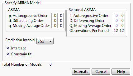
Shows the ARIMA Model Group window, which enables you to fit a range of ARIMA or Seasonal ARIMA models by specifying the range of orders. As you enter ranges into the window, the Total Number of Models updates accordingly.

Figure 18.8 ARIMA Model Group Specification Window 

Once you specify the models and click Estimate, a Model Report for each specified model is added to the report window. See Additional Time Series Reports.

Simple Smoothing Average Specification Window

The Simple Smoothing Average Specification window appears when you select Simple Moving Average as the smoothing model. Let w be the smoothing window width in a simple moving average (SMA) model. Let ft=(yt+yt-1+yt-2+...+yt-(w-2)+yt-(w-1))/w be the average of w consecutive observations for some time point t.

Figure 18.9 Simple Smoothing Average Specification Window 

Enter smoothing window width

The smoothing window width, w, that defines the number of consecutive points to average. The larger the window width, the more the series is smoothed.

No Centering

The smoothing window is constructed from the points leading up to and including the time point, t, the point at which the series is being estimated. In other words, ft is the plotted value for time t.

Centered

The smoothing window is centered around the time point at which the series is being estimated.

– For odd w, ft is the plotted value for time t-(w-1)/2.

– For even w, ft is the plotted value for time t-(w-1)/2. When saved to a data table, ft is at t-(w-2)/2.

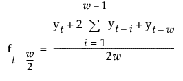
Centered and Double Smoothed for Even Number of Terms

For even w, the smoothing window cannot be centered around the time point at which the series is being estimated. This option creates two smoothing windows that are almost centered, and averages them together. The smoothing estimates are calculated as follows:

Smoothing Model Windows

The Smoothing Model specification windows appear when you select one of the smoothing model options other than Simple Moving Average. The title of the window and the available options depend on the smoothing model option that you select.

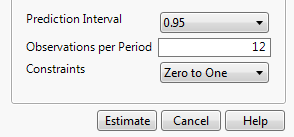
Figure 18.10 Smoothing Model Specification Window 

Prediction Interval

Enables you to set the prediction level for the forecast prediction intervals.

Observations per Period

(Available only for seasonal smoothing models.) Enables you to set the number of observations per period in a seasonal smoothing model.

Constraints

Enables you to specify what type of constraint you want to enforce on the smoothing weights during the fit. The following constraint options are available:

Zero To One

Constrains the values of the smoothing weights to the range zero to one.

Unconstrained

Allows the parameters to range freely.

Stable Invertible

Constrains the parameters such that the equivalent ARIMA model is stable and invertible.

Custom

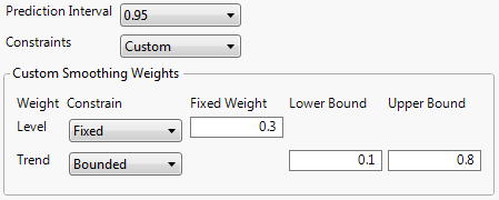
Expands the dialog to enable you to set constraints on individual smoothing weights. Each smoothing weight can be Bounded, Fixed, or Unconstrained as determined by the setting of the popup menu next to the weight’s name. When entering values for fixed or bounded weights, the values can be positive or negative real numbers.

Figure 18.11 Custom Smoothing Weights 

The example shown in Figure 18.11 has the Level weight (α) fixed at a value of 0.3 and the Trend weight (γ) bounded by 0.1 and 0.8. In this case, the value of the Trend weight is allowed to move within the range 0.1 to 0.8 while the Level weight is held constant at 0.3. Note that you can specify all the smoothing weights in advance by using these custom constraints. In that case, none of the weights would be estimated from the data although forecasts and residuals would still be computed.